Introduction 00:00

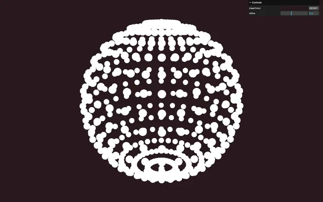
A rather difficult technique I get questions about, is the field of particles you can see on Chartogne Taillet website:

Particles seem to move as if they are influenced by various streams pushing them around. There are actually two techniques implemented:

• GPGPU
• Flow field

We are going to explain both techniques and apply them in order to animate the following model https://sketchfab.com/3d-models/mv-spartan-e2c3ced464f14e3b864f15871bf6d87d

Setup 02:10

The starter is quite similar to the previous lesson with particles ready to be enhanced:

• A tweakable clearColor
• A model file named model.glb that you can find in the static/ folder (you can download the original Blender file using the Resources button)
• A GLTFLoader instance with a DracoLoader instance associated with it
• A sphere made out of particles using a ShaderMaterial
• The vite-plugin-glsl dependency to handle GLSL files
• OrbitControls to rotate around

Regarding the particles shader:

• The size is already handled with perspective and we can control it using the uSize tweak
• Particles are shaped as discs
• The color is sent from the vertex to the fragment as the vColor varying

Theory 03:44

GPGPU and flow field, what’s the difference?

GPGPU stands for General-Purpose computing on Graphics Processing Units. It’s a way of using the GPU to process data rather than rendering pixels for the end-user. It’s great for when you need to do the same complex calculation thousands of times.

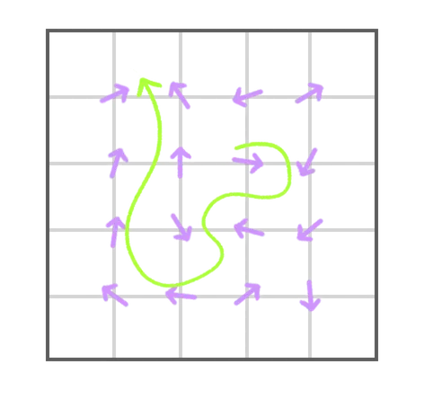
Flow field corresponds to spatialized streams. For any point in space, we calculate a direction:

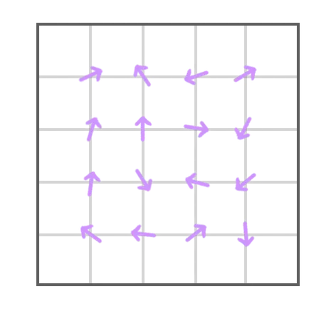
Now imagine throwing a particle on a flow field. For each frame, we would calculate the stream direction for the particle and make it move accordingly, resulting in the particle moving around:

Unfortunately, a flow field takes up a considerable amount of computing power. As a result, doing the calculation for each frame for thousands and thousands of particles using just the CPU wouldn’t be possible, which is why we are going to use the aforementioned GPGPU.

Persistence

An important aspect of the problem is that the data needs to persist. Until now, when doing animation on particles, we have been calculating a sort of snapshot of where all particles should be.

In the case of a flow field, the trajectory of the particle is unpredictable and keeps on evolving with time. We need to save the current position of all particles to use it on the next frame.

We can’t save the result in the attribute because updating would result in a catastrophic frame rate if used on too many particles.

And this is where the GPGPU solves our problem perfectly. As mentioned earlier, GPGPU helps us process data using the GPU. To do that, it utilizes what we call FBO (Frame Buffer Object).

FBOs are textures in which we save the renders instead of doing it on the <canvas> and they can be created in Three.js using WebGLRenderTarget.

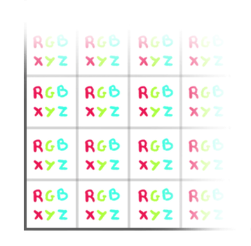
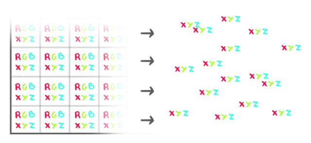
In the case of particles, we use each pixel of the texture for one particle where the RGB channels correspond to the XYZ coordinates. And the A channel can be used for something else if we need (which we are going to need):

Instead of using the classic position attribute on the particles vertex shader, we use the FBO generated and updated by the GPGPU:

On each frame, we update the FBO according to the previous FBO. This way, the position of the particles persists and we keep on updating them.

Creating our own GPGPU

Although it may seem very interesting, creating our own GPGPU is quite daunting. We are going to use a solution that will save us a lot of time and headaches. Yet, it’s important to understand the technique in order to use it properly, allowing us to achieve the best result possible.

Here’s how it would go if we were to do it ourselves.

First, we need to create a brand new offscreen scene. This scene is independent from the actual scene that the user sees.

In it, we put a camera facing a plane which fills the camera view perfectly.

To that plane, we apply a custom shader. To that custom shader, we send the FBO texture containing the position of the particles. But instead of just displaying the texture, the custom shader updates the pixels, thus updating the particles.

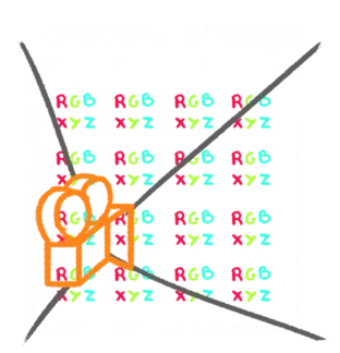
And this is where we calculate and apply the flow field to the pixels as if the RGB channels were XYZ coordinates.

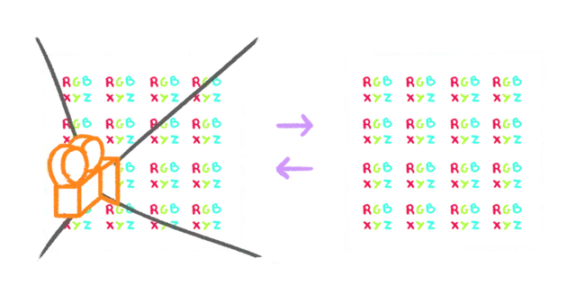
Then, before rendering the real scene, we render that offscreen scene using the offscreen camera and save the result in an FBO.

For the next frame, we send the result of the previously rendered FBO to the plane shader and complete a new render while applying the flow field again to the pixels.

And again for the next frame. And again, and again.

We end up with an FBO (a texture) containing the particle coordinates, while the pixels are being updated for each frame. These updates are done in the blink of an eye thanks to the GPU.

This is the theory; unfortunately, it’s even more complex.

First, we can’t read and write in the same FBO, which is why we need to have two of them and to invert them on each new update. We call this way of doing things the “ping-pong buffers”.

Secondly, using pixel as data is difficult because of the various formats and types a pixel can have.

Finally, we need to complete the setup with almost nothing on screen until it works. This is why debugging a GPGPU is very complex.

GPUComputationRenderer to the rescue

Fortunately, there is a Three.js class to solve that issue.

GPUComputationRenderer will do most of the heavy lifting such as creating the scene, handling the ping-pong buffers, setting the color format properly, rendering, etc.

As I’m writing, the class isn’t well documented and there is actually no page in the Three.js documentation.

Fortunately, the code is well commented: GPUComputationRenderer.js

And there are some examples: https://threejs.org/examples/?q=gpgpu#webgl_gpgpu_birds

Anyway, you’re going to learn how to use it here.

GPGPU 21:49

We are going to setup the GPGPU and test it on this simple sphere for now. Later, we will switch to the boat model.

Be careful and try not to stray from the lesson, at least until you get the particles moving. Even though GPUComputationRenderer makes things easier, there is a lot of coding ahead.

Geometry

First, we need to make minor changes to the structure of our code.

We want to instantiate the GPUComputationRenderer, but the very first parameters are the width and height. This size will be used internally to create the FBOs and it depends on the amount of particles because we need one pixel per particle.

We know the amount of particles thanks to the geometry, which is why we are going to declare the geometry before the rest.

Right before the Particles section, create a Base geometry section and create a baseGeometry object:

/**
 * Base geometry
 */
const baseGeometry = {}

/**
 * Particles
 */
// ...

Put the SphereGeometry instance in an instance property:

const baseGeometry = {}
baseGeometry.instance = new THREE.SphereGeometry(3)

Save the amount of particles as the count property, using baseGeometry.instance.attributes.position.count:

const baseGeometry = {}
baseGeometry.instance = new THREE.SphereGeometry(3)
baseGeometry.count = baseGeometry.instance.attributes.position.count

In the Particles section, remove the particles.geometry and use the baseGeometry.instance on the Points:

/**
 * Particles
 */
const particles = {}

// Material
// ...

// Points
particles.points = new THREE.Points(baseGeometry.instance, particles.material)
scene.add(particles.points)

We get the exact same result, but between the Base geometry and the Particles sections, we are going to set up our GPUComputationRenderer.

GPUComputationRenderer

Right before the Particles section, create a GPU Compute section with a gpgpu object:

/**
 * GPU Compute
 */
// Setup
const gpgpu = {}

We use objects to organise and separate things.

We want to instantiate the GPUComputationRenderer. Import it from three/addons/misc/GPUComputationRenderer.js:

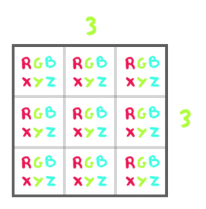
import { GPUComputationRenderer } from 'three/addons/misc/GPUComputationRenderer.js'

Remember that each pixel of the FBOs will correspond to one particle. Let me give you an example: if we have 9 particles, we need 9 pixels on the FBOs. Since FBOs are like 2D renders, they are rectangular. In order to make calculations easier, we are going to consider them as squares.

For 9 particles, we need a 3 by 3 FBO and we can calculate that thanks to the square root.

The square root of 9 equals 3:

But what about 10 particles?

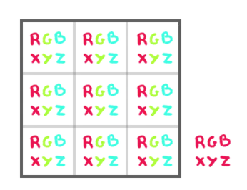
The square root of 10 equals 3.1622. We need a round number, and we can round it up to 4 so that each particle fits:

We get some left-over pixels, but it’s not much of an issue.

Create a size property and assign to it the result of Math.ceil() of the Math.sqrt() of baseGeometry.count:

const gpgpu = {}
gpgpu.size = Math.ceil(Math.sqrt(baseGeometry.count))

We can instantiate the GPUComputationRenderer and assign it to a computation property. The first two parameters are the width and height, which is gpgpu.size for both (it’s a square). The third parameter is the renderer:

const gpgpu = {}
gpgpu.size = Math.ceil(Math.sqrt(baseGeometry.count))
gpgpu.computation = new GPUComputationRenderer(gpgpu.size, gpgpu.size, renderer)

Base positions

To that GPUComputationRenderer, we need to send the base particles as a texture. It’s the base texture that will be used for the first render and then updated again and again.

We can create one texture using the createTexture() method:

// Base particles
const baseParticlesTexture = gpgpu.computation.createTexture()

Let’s have a look inside with a console.log():

const baseParticlesTexture = gpgpu.computation.createTexture()
console.log(baseParticlesTexture)

It’s a DataTexture which is similar to other Three.js textures but the pixels data is set up as an array which we can access in baseParticlesTexture.image.data:

const baseParticlesTexture = gpgpu.computation.createTexture()
console.log(baseParticlesTexture.image.data)

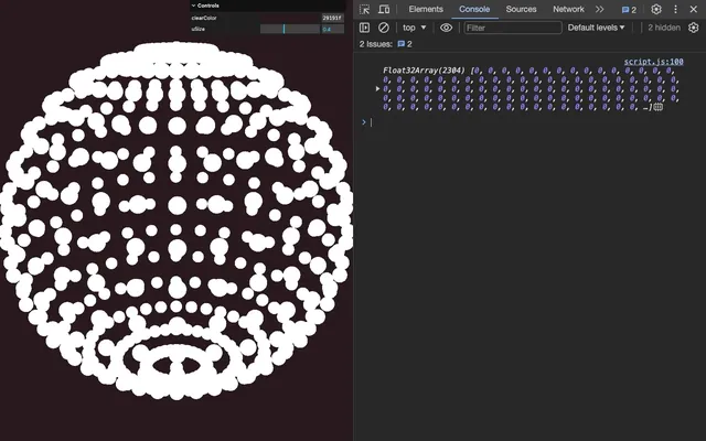
We get a bunch of 0. Each set of 4 values will correspond to one particle because each set of 4 values are the r, g, b and a channels of one pixel.

Let’s keep the baseParticlesTexture like this for now, and later, we are going to put the particles positions in there instead of those 0.

Particles variable

GPUComputationRenderer works in a way where each type of data that will be computed is called a “variable”. In our case, we have only one variable and it’s the particles.

To create a variable, we send the base texture (baseParticlesTexture) that we created earlier. In addition, we need to send a shader that will update that texture.

Let’s create the shader. In src/shaders/, create a gpgpu/ folder. In that gpgpu/ folder, create a particles.glsl file and add the minimal fragment shader code to paint each pixel red:

void main()
{
    gl_FragColor = vec4(1.0, 0.0, 0.0, 1.0);
}

Yes, this means that, currently, all the particles are at the 1.0, 0.0, 0.0 coordinates.

Back to the script.js: import the shader as gpgpuParticlesShader:

import gpgpuParticlesShader from './shaders/gpgpu/particles.glsl'

Create a “variable” using the addVariable() method, send 'uParticles' as the first parameter, the gpgpuParticlesShader shader as the second parameter and the baseParticlesTexture as the third parameter. Save it in gpgpu.particlesVariable:

// Base particles
const baseParticlesTexture = gpgpu.computation.createTexture()

// Particles variable
gpgpu.particlesVariable = gpgpu.computation.addVariable('uParticles', gpgpuParticlesShader, baseParticlesTexture)

'uParticles' is the name we choose for the texture. This means that, in the shader we provided, we can access the texture as uParticles.

As mentioned earlier, we want the particles to persist in time, meaning that their coordinates will be saved and re-used in the next frame.

The “variable” needs to be re-injected into itself. To do that, we can use the setVariableDependencies() method.

The first parameter is the variable (gpgpu.particlesVariable in our case) and the second parameter is an array containing the dependencies (the same gpgpu.particlesVariable):

// Particles variable
gpgpu.particlesVariable = gpgpu.computation.addVariable('uParticles', gpgpuParticlesShader, baseParticlesTexture)
gpgpu.computation.setVariableDependencies(gpgpu.particlesVariable, [ gpgpu.particlesVariable ])

This is how we create a loop, which allows us to keep on sending and updating the same texture.

Our GPUComputationRenderer is ready and we can initialize it with the init() method:

// Init
gpgpu.computation.init()

We now want to update our particles variable on each frame and it’s as simple as calling the compute() method on the GPUComputationRenderer instance, in the tick function, before the final render:

const tick = () =>
{
    // ...

    // GPGPU Update
    gpgpu.computation.compute()

    // Render normal scene
    // ...
}

Debug

That was a lot of coding, it’s probably still fuzzy, and we still haven’t seen anything on screen.

Before trying to use the output of GPUComputationRenderer on the particles, we are going to test what’s in there.

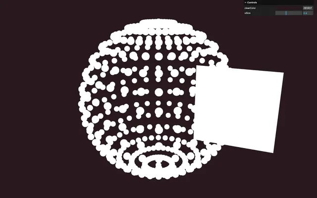
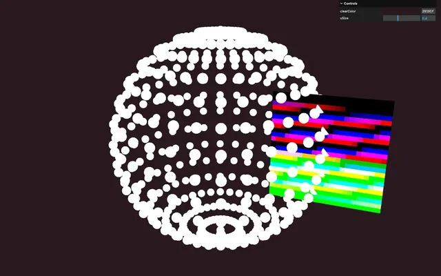
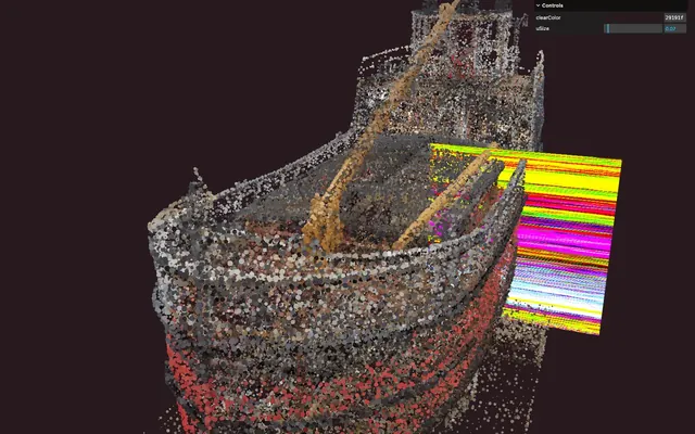
In the end, what we want from GPUComputationRenderer is a texture containing the particles coordinates. We are going to create a plane and apply the GPUComputationRenderer output texture to it, just to see what we get.

Back to the GPU Compute section: create a debug plane using PlaneGeometry and MeshBasicMaterial, move it sideways and add it to the scene:

// Debug
gpgpu.debug = new THREE.Mesh(
    new THREE.PlaneGeometry(3, 3),
    new THREE.MeshBasicMaterial()
)
gpgpu.debug.position.x = 3
scene.add(gpgpu.debug)

We want to apply the GPUComputationRenderer output texture to that plane and we can access it using the getCurrentRenderTarget(). To this method, we need to send the variable, which is gpgpu.particlesVariable in our case.

console.log() it, out of curiosity:

console.log(gpgpu.computation.getCurrentRenderTarget(gpgpu.particlesVariable))

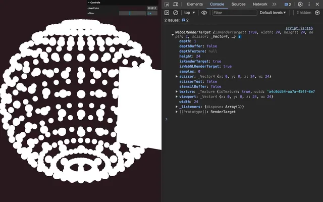
We get a WebGLRenderTarget which is the Three.js class handling the FBO.

We can access the actual texture using the texture property:

console.log(gpgpu.computation.getCurrentRenderTarget(gpgpu.particlesVariable).texture)

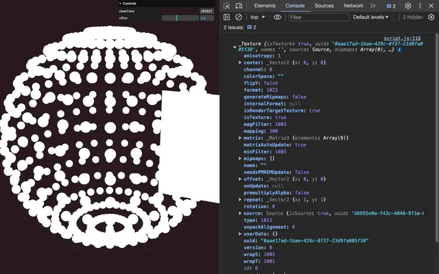
And we can assign that texture to the map property of the MeshBasicMaterial:

gpgpu.debug = new THREE.Mesh(
    new THREE.PlaneGeometry(3, 3),
    new THREE.MeshBasicMaterial({ map: gpgpu.computation.getCurrentRenderTarget(gpgpu.particlesVariable).texture })
)
gpgpu.debug.position.x = 3
scene.add(gpgpu.debug)

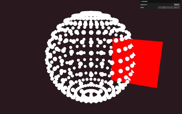
We get a fully red plane because our particles.glsl shader only outputs red, which is fine, for now.

Send and update the particles

Instead of that uniform red, we want to have our particles as pixels. We already sent baseParticlesTexture to the shader when creating the particles variable, but it’s currently filled with a bunch of 0. Let’s populate it.

We want to configure each particle's coordinates (x, y and z) as the r, g and b channels and ignore the a channel for now.

Right after creating the baseParticlesTexture, use a classic for(…) to loop from 0 to baseGeometry.count:

// Base particles
const baseParticlesTexture = gpgpu.computation.createTexture()

for(let i = 0; i < baseGeometry.count; i++)
{
}

The geometry particles are located in baseGeometry.instance.attributes.position.array and go 3 by 3 because x, y and z.

The array we need to update is located in baseParticlesTexture.image.data and the values go 4 by 4 because r, g, b and a.

We need an i3 and an i4:

for(let i = 0; i < baseGeometry.count; i++)
{
    const i3 = i * 3
    const i4 = i * 4
}

We can now put the values from baseGeometry.instance.attributes.position.array to baseParticlesTexture.image.data using i3 and i4 respectively and set the fourth value (the alpha) to 0 for now:

for(let i = 0; i < baseGeometry.count; i++)
{
    const i3 = i * 3
    const i4 = i * 4

    // Position based on geometry
    baseParticlesTexture.image.data[i4 + 0] = baseGeometry.instance.attributes.position.array[i3 + 0]
    baseParticlesTexture.image.data[i4 + 1] = baseGeometry.instance.attributes.position.array[i3 + 1]
    baseParticlesTexture.image.data[i4 + 2] = baseGeometry.instance.attributes.position.array[i3 + 2]
    baseParticlesTexture.image.data[i4 + 3] = 0
}

Have a look at the baseParticlesTexture.image.data using a console.log() and you should have 3 values, then a 0, again and again:

const baseParticlesTexture = gpgpu.computation.createTexture()

for(let i = 0; i < baseGeometry.count; i++)
{
    // ...
}
console.log(baseParticlesTexture.image.data)

The very last values are at 0 because the pixels aren’t associated with particles.

In the particles.glsl, we now want to retrieve the texture. We opted for the name 'uParticles' and the GPUComputationRenderer automatically injected the texture as a sampler2D uParticles.

But now, we want to pick the color from that uParticles.

We need the classic UV coordinates and we can get them using the following formula gl_FragCoord.xy / resolution.xy.

We’ve seen gl_FragCoord.xy in the Halftone lesson. It’s the screen coordinates and it corresponds to the pixel starting from the bottom left:

resolution.xy contains the size of the render and since we use it to divide gl_FragCoord.xy, we get 0 to 1 UV coordinates.

Save it as a float uv variable at the start of main():

void main()
{
    vec2 uv = gl_FragCoord.xy / resolution.xy;
    gl_FragColor = vec4(1.0, 0.0, 0.0, 1.0);
}

Send it as the first values of gl_FragColor and keep the other values at 1.0:

void main()
{
    vec2 uv = gl_FragCoord.xy / resolution.xy;
    gl_FragColor = vec4(uv, 1.0, 1.0);
}

We get the classic UV coordinates and we can use them to pick the color from uPosition with the texture() function:

void main()
{
    vec2 uv = gl_FragCoord.xy / resolution.xy;
    vec4 particle = texture(uParticles, uv);
    gl_FragColor = vec4(uv, 1.0, 1.0);
}

Send the whole result to gl_FragColor:

void main()
{
    vec2 uv = gl_FragCoord.xy / resolution.xy;
    vec4 particle = texture(uParticles, uv);
    gl_FragColor = particle;
}

Although it might look buggy, each square of the plane corresponds to one pixel of the uParticles texture which, itself, corresponds to the coordinates of each particle.

And the cool part is that the data is persisting, meaning that if we update particle, we will get the updated version in the next frame and we can keep on updating it.

As an example add 0.01 to the y property:

void main()
{
    vec2 uv = gl_FragCoord.xy / resolution.xy;
    vec4 particle = texture(uParticles, uv);
    particle.y += 0.01;
    gl_FragColor = particle;
}

The pixels become more green. Since green corresponds to the y coordinate, it means that the particles would go up.

Note that rgba and xyzw are interchangeable. You can use one or the other and have the same effect. But since we consider the pixels as particles, it makes sense to use xyz.

After a few seconds, the pixels stop changing and you might think that the particles will also stop moving, but the value actually keeps on getting higher. It’s just that the color channels are visually confined to the range between 0 to 1.

Use the GPGPU to position particles 01:01:44

Our GPGPU, even though very basic, is ready and we now want to use that texture to position the particles.

Currently, the particles are using the baseGeometry.instance as the geometry when instantiating the Points, but we want to use the GPGPU texture instead.

Let’s start from an empty geometry. In the Particles section, create a BufferGeometry, save it as particles.geometry and send it to the Points:

/**
 * Particles
 */
// ...

// Geometry
particles.geometry = new THREE.BufferGeometry()

// ...

// Points
particles.points = new THREE.Points(particles.geometry, particles.material)
scene.add(particles.points)

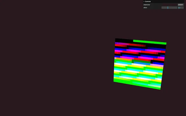
The particles are gone.

By default, Three.js uses the amount of items in the position attribute to know how many points to draw. However, we don’t want to rely on the position attribute anymore.

Fortunately, we can use the setDrawRange() method on the geometry to define a range of vertices:

// Geometry
particles.geometry = new THREE.BufferGeometry()
particles.geometry.setDrawRange(0, baseGeometry.count)

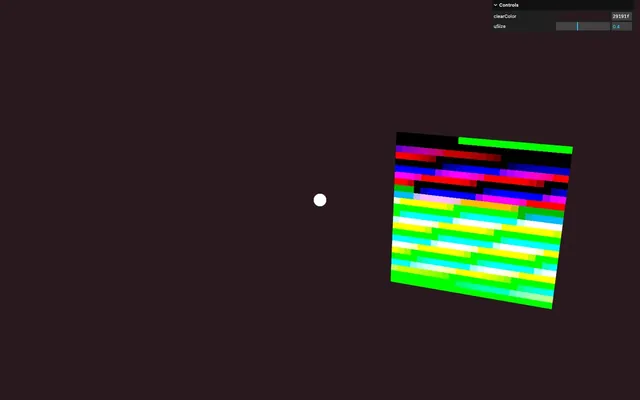
There are currently thousands of particles at the center of the scene and we are going to use the GPGPU to move them.

In the ShaderMaterial, send a uParticlesTexture uniform using the Uniform class and keep it empty for now:

particles.material = new THREE.ShaderMaterial({
    // ...
    uniforms:
    {
        // ...
        uParticlesTexture: new THREE.Uniform()
    }
})

In the tick function, update the uParticlesTexture uniform using the same technique we used previously to access the FBO from the GPGPU with the getCurrentRenderTarget() method and don’t forget that it’s the texture property we want:

const tick = () =>
{
    // ...

    // GPGPU Update
    gpgpu.computation.compute()
    particles.material.uniforms.uParticlesTexture.value = gpgpu.computation.getCurrentRenderTarget(gpgpu.particlesVariable).texture

    // ...
}

We need to send the RenderTarget texture on each frame because GPUComputationRenderer is using multiple FBOs for the ping-pong buffers, and we need the current one that has been used when computing this frame.

In the vertex shader of the particles, we want to pick the texture from the uParticlesTexture like we did in particles.glsl, but this time around, we cannot do it using gl_FragCoord.xy since those are screen coordinates.

Instead, we are going to send the UV coordinates ourselves as an attribute.

In the Geometry part of the Particles, before creating the BufferGeometry, create a particlesUvArray array using a Float32Array of length baseGeometry.count * 2:

// Geometry
const particlesUvArray = new Float32Array(baseGeometry.count * 2)

particles.geometry = new THREE.BufferGeometry()

We now want to fill the particlesUvArray with UV coordinates corresponding to the pixels in the uParticlesTexture.

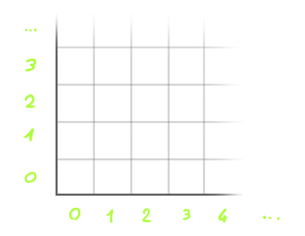
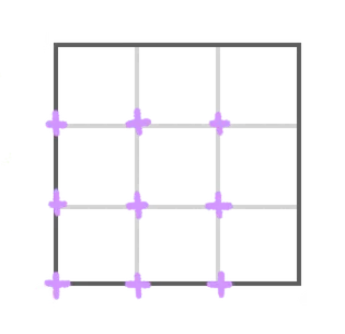
To understand the following part, here are the coordinates we would need if we had 9 particles (3 by 3):

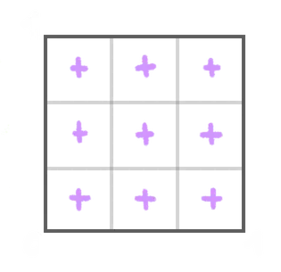
The purple crosses are at the center of each cell.

To get there, we are going to do a first … for … loop for the y coordinate (the rows) and inside that … for … loop, we are going to do a second … for … loop for the x coordinate (the columns):

const particlesUvArray = new Float32Array(baseGeometry.count * 2)

for(let y = 0; y < gpgpu.size; y++)
{
    for(let x = 0; x < gpgpu.size; x++)
    {
    }
}

In there, we still need to have access to an index going from 0 to the amount of particles and we can do that by multiplying y by gpgpu.size and adding x. Save the result as i:

for(let y = 0; y < gpgpu.size; y++)
{
    for(let x = 0; x < gpgpu.size; x++)
    {
        const i = (y * gpgpu.size + x)
    }
}

And since we need two values per vertex when filling particlesUvArray, let’s calculate a i2 by multiplying i by 2:

for(let y = 0; y < gpgpu.size; y++)
{
    for(let x = 0; x < gpgpu.size; x++)
    {
        const i = (y * gpgpu.size + x)
        const i2 = i * 2
    }
}

Currently, x and y are going from 0 to gpgpu.size, but we need them to go from 0 to 1 (not included) since we want UV coordinates.

To do that, create a uvX and a uvY variables and divide x and y by gpgpu.size:

for(let y = 0; y < gpgpu.size; y++)
{
    for(let x = 0; x < gpgpu.size; x++)
    {
        const i = (y * gpgpu.size + x)
        const i2 = i * 2

        const uvX = x / gpgpu.size
        const uvY = y / gpgpu.size
    }
}

We are almost there, unfortunately, those uvX and uvY coordinates are not in the middle of the cells. Instead, they are currently at the bottom left corner:

To fix that, all we need to do is add 0.5 to the x and y before dividing by gpgpu.size:

for(let y = 0; y < gpgpu.size; y++)
{
    for(let x = 0; x < gpgpu.size; x++)
    {
        const i = (y * gpgpu.size + x)
        const i2 = i * 2

        // Particles UV
        const uvX = (x + 0.5) / gpgpu.size
        const uvY = (y + 0.5) / gpgpu.size
    }
}

And that’s it. We can now save uvX and uvY in particlesUvArray respectively at the i2 and i2 + 1 indices:

for(let y = 0; y < gpgpu.size; y++)
{
    for(let x = 0; x < gpgpu.size; x++)
    {
        const i = (y * gpgpu.size + x)
        const i2 = i * 2

        // Particles UV
        const uvX = (x + 0.5) / gpgpu.size
        const uvY = (y + 0.5) / gpgpu.size

        particlesUvArray[i2 + 0] = uvX;
        particlesUvArray[i2 + 1] = uvY;
    }
}

After the setDrawRange(), create a new attribute using the setAttribute() method, name it 'aParticlesUv' and set the BufferAttribute size to 2:

particles.geometry = new THREE.BufferGeometry()
particles.geometry.setDrawRange(0, baseGeometry.count)
particles.geometry.setAttribute('aParticlesUv', new THREE.BufferAttribute(particlesUvArray, 2))

In particles/vertex.glsl, retrieve the uParticlesTexture uniform as a sampler2D and the aParticlesUv attribute as vec2:

uniform sampler2D uParticlesTexture;

attribute vec2 aParticlesUv;

We can now pick the color from uParticlesTexture using texture() at the aParticlesUv coordinates:

void main()
{
    vec4 particle = texture(uParticlesTexture, aParticlesUv);
    
    // ...
}

Next, use it for the modelPosition instead of position by swizzling the xyz since we only want the position:

void main()
{
    vec4 particle = texture(uParticlesTexture, aParticlesUv);

    // Final position
    vec4 modelPosition = modelMatrix * vec4(particle.xyz, 1.0);
    // ...
}

The particles positions are now entirely controlled from the GPGPU, more precisely from the particles.glsl shader.

You can try that in gpgpu/particles.glsl by changing particle.y += by particle.x +=:

void main()
{
    // ...
    particle.x += 0.01;
    // ...
}

Instead of that lame transition, we are going to implement the flow field. But we need some more preparation first.

Use a model 01:21:35

We are going to use the model you can find on SketchFab: https://sketchfab.com/3d-models/mv-spartan-e2c3ced464f14e3b864f15871bf6d87d

It’s a mesh reconstruction based on photos. We call this technique photogrammetry.

The model is under CCO license with a decent amount of vertices.

I imported it in Blender, transformed it a little and baked the texture into the vertex color.

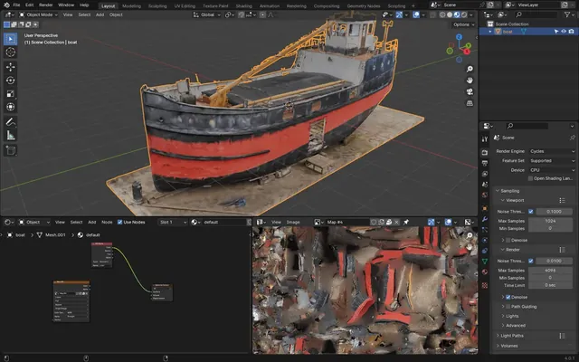
You can find the modified version in the Blender files using the Resources button.

Load

We are going to load the model and use its geometry instead of SphereGeometry. As you know, loading models takes time. This means that we need to wait for the model to load before initializing the GPGPU and the particles.

We are going to end up with a lot of code in the callback function, but there is actually a trick named “async loading” which will get us rid of the callback function.

Before the Base Geometry section, load the model using the following instruction and console.log() the result:

/**
 * Load model
 */
const gltf = await gltfLoader.loadAsync('./model.glb')
console.log(gltf)

We get the gltf immediately without any callback function.

What’s going on here is that we are using the loadAsync() which returns a Promise. In fact, we ask our code to wait for the Promise to be resolved before going any further using the await keyword.

Promises, await and async are part of a whole new and complex topic which we are not going to cover here, but the way to use it is as simple as demonstrated right now.

One thing to understand is that using await here is made possible thanks to Vite which creates an async scope allowing us to use the await at the top level. If you try to build the project using npm run build or try to put it live using Vercel (which will also rely on npm run build), you’ll very likely get an error because Vite tries to make your project compatible with most browsers, and top-level await isn’t available on all targeted browsers for compatibility.

To fix that, we can simply change the browsers targeted list. In the vite.config.js file, in the build property, add target: 'esnext':

export default {
    // ...
    build:
    {
        // ...
        target: 'esnext'
    },
    // ...
}

Your build should now work, but Vite won’t try to transpile down to old browsers, which should be fine.

Another drawback is that, if the model takes time to load, the code will be stuck here for a while and the user won’t be able to see anything in the meantime.

As far as experiments with lightweight models are concerned, it’s okay, but otherwise, you should use more adapted solutions, which I cover in the Code structuring for bigger projects lesson.

Regardless, we now have our loaded model as gltf and we can extract the geometry from the first and only child of the scene. Then, we save it in baseGeometry.instance instead of the SphereGeometry:

/**
 * Base geometry
 */
const baseGeometry = {}
baseGeometry.instance = gltf.scene.children[0].geometry

We get our boat, but the particles are too big. Lower uSize to 0.07:

particles.material = new THREE.ShaderMaterial({
    // ...
    uniforms:
    {
        uSize: new THREE.Uniform(0.07),
        // ...
    }
})

Colors

As mentioned earlier, I’ve saved the color directly in vertex colors which we can access using baseGeometry.instance.attributes.color.

Right after setting the 'aParticlesUv' attribute, we can set a new attribute named 'aColor' and send baseGeometry.instance.attributes.color which is already a BufferAttribute:

particles.geometry.setAttribute('aParticlesUv', new THREE.BufferAttribute(particlesUvArray, 2))
particles.geometry.setAttribute('aColor', baseGeometry.instance.attributes.color)

In particles/vertex.glsl, retrieve the aColor attribute as a vec3 and forward it to the vColor:

// ...
attribute vec3 aColor;

// ...

void main()
{
    // ...
    vColor = aColor;
}

Randomized size

Since we are in the attributes, let’s randomize the size of the particles.

After creating the particlesUvArray, create a sizesArray array using a Float32Array of size baseGeometry.count:

// Geometry
const particlesUvArray = new Float32Array(baseGeometry.count * 2)
const sizesArray = new Float32Array(baseGeometry.count)

In the double … for … where we populated the particlesUvArray array, fill the sizesArray with a bunch of Math.random() at the i index since we only have one value per vertex:

for(let y = 0; y < gpgpu.size; y++)
{
    for(let x = 0; x < gpgpu.size; x++)
    {
        // ...

        // Size
        sizesArray[i] = Math.random()
    }
}

Set a new attribute named 'aSize', use a BufferAttribute, send it sizesArray and set its item size to 1:

particles.geometry.setAttribute('aSize', new THREE.BufferAttribute(sizesArray, 1))

In particles/vertex.glsl, retrieve the aSize attribute as a float and multiply it in the gl_PointSize:

// ...
attribute float aSize;

// ...

void main()
{
    // ...

    // Point size
    gl_PointSize = aSize * uSize * uResolution.y;
    gl_PointSize *= (1.0 / - viewPosition.z);

    // ...
}

Flow field animation 01:36:19

Setting up the GPGPU took a lot of preparation, but now, we are ready to create the flow field and replace this boring animation.

As mentioned earlier, a flow field corresponds to a spatialized stream. For any 3D point, we calculate a direction and we use that direction to move the particle. Some will go in one direction, while others will go in different directions. To make those directions feel natural and vary smoothly, we are going to use the Simplex Noise we discovered in previous lessons.

And since the Simplex Noise allows more than 3 dimensions, we are going to use a 4D Simplex Noise in order to make the streams vary in time too.

The 4D Simplex Noise is already available in the src/shaders/includes/simplexNoise4d.glsl and has been taken from the usual Gist: https://gist.github.com/patriciogonzalezvivo/670c22f3966e662d2f83

In gpgpu/particles.glsl, remove the particle.x += 0.01;:

void main()
{
    vec2 uv = gl_FragCoord.xy / resolution.xy;
    vec4 particle = texture(uParticles, uv);
    gl_FragColor = particle;
}

Before the main(), include simplexNoise4d.glsl:

#include ../includes/simplexNoise4d.glsl

void main()
{
    // ...
}

Since a flow field is a 3D direction, we are going to create a vec3 flowField (don’t save yet):

void main()
{
    vec2 uv = gl_FragCoord.xy / resolution.xy;
    vec4 particle = texture(uParticles, uv);

    // Flow field
    vec3 flowField = vec3();

    gl_FragColor = particle;
}

Call simplexNoise4d() on each one of the 3 axes of the vec3() and send a vec4() to each one because it’s a 4D Simplex Noise (don’t save yet):

void main()
{
    vec2 uv = gl_FragCoord.xy / resolution.xy;
    vec4 particle = texture(uParticles, uv);

    // Flow field
    vec3 flowField = vec3(
        simplexNoise4d(vec4()),
        simplexNoise4d(vec4()),
        simplexNoise4d(vec4())
    );

    gl_FragColor = particle;
}

For the first 3 values of the vec4(), we are going to use the particle position by swizzling the xyz and for the fourth value, we are setting it to 0.0 for now:

void main()
{
    vec2 uv = gl_FragCoord.xy / resolution.xy;
    vec4 particle = texture(uParticles, uv);
    
    // Flow field
    vec3 flowField = vec3(
        simplexNoise4d(vec4(particle.xyz, 0.0)),
        simplexNoise4d(vec4(particle.xyz, 0.0)),
        simplexNoise4d(vec4(particle.xyz, 0.0))
    );

    gl_FragColor = particle;
}

Since it’s a direction, let’s normalize it so that its length is always 1:

void main()
{
    // ...
    
    // Flow field
    vec3 flowField = vec3(
        simplexNoise4d(vec4(particle.xyz, 0.0)),
        simplexNoise4d(vec4(particle.xyz, 0.0)),
        simplexNoise4d(vec4(particle.xyz, 0.0))
    );
    flowField = normalize(flowField);

    // ...
}

Moving the particle is as simple as adding the flowField to the particle.xyz:

void main()
{
    // ...
    
    // Flow field
    vec3 flowField = vec3(
        simplexNoise4d(vec4(particle.xyz, 0.0)),
        simplexNoise4d(vec4(particle.xyz, 0.0)),
        simplexNoise4d(vec4(particle.xyz, 0.0))
    );
    flowField = normalize(flowField);
    particle.xyz += flowField;

    // ...
}

Not the expected result. We have a few problems to solve.

First, all the particles are moving in a diagonal direction because we are sending the same coordinates to the three simplexNoise4d().

We need to send different values, and we can simply offset them slightly:

void main()
{
    // ...
    
    // Flow field
    vec3 flowField = vec3(
        simplexNoise4d(vec4(particle.xyz + 0.0, 0.0)),
        simplexNoise4d(vec4(particle.xyz + 1.0, 0.0)),
        simplexNoise4d(vec4(particle.xyz + 2.0, 0.0))
    );

    // ...
}

Now the effect is too strong.

Lower it by multiplying flowField by 0.01 when applying it to the particle.xyz:

void main()
{
    // ...
    particle.xyz += flowField * 0.01;

    // ...
}

And now we get something looking like a flow field, but after a few seconds, particles seem stuck in loops.

It’s because the flow field stays the same in time and particles end up following the same path. We want to make the Simplex Noise vary in time. This is exactly what the fourth value of the vec4 can be used for. But since we want it to vary with the time, we need to send that time to the shader.

We want to add a uTime uniform, but be careful, as we want to set it on the GPGPU variable handling the particles, not the final particles ShaderMaterial.

To do that, you can access the GPGPU ShaderMaterial handling the particles using gpgpu.particlesVariable.material and it works like any ShaderMaterial, meaning that it has a uniforms property.

On gpgpu.particlesVariable.material.uniforms, add a uTime uniform using Uniform and set it to 0:

// Particles variable
gpgpu.particlesVariable = gpgpu.computation.addVariable('uParticles', gpgpuParticlesShader, baseParticlesTexture)
gpgpu.computation.setVariableDependencies(gpgpu.particlesVariable, [ gpgpu.particlesVariable ])

// Uniforms
gpgpu.particlesVariable.material.uniforms.uTime = new THREE.Uniform(0)

In tick, update its value using the elapsedTime, before the compute():

const tick = () =>
{
    // ...

    // GPGPU Update
    gpgpu.particlesVariable.material.uniforms.uTime.value = elapsedTime
    gpgpu.computation.compute()
    // ...
}

Back to gpgpu/particles.glsl: retrieve the uTime uniform as a float:

uniform float uTime;

uTime is going to be a bit fast for what we want to do. Since we are going to use it in multiple places within the code, let’s create a variable for it.

At the beginning of main(), create a float time variable and assign to it uTime multiplied by 0.2:

void main()
{
    float time = uTime * 0.2;
    // ...
}

Use it as the fourth value of the simplexNoise4d() instead of the 0.0:

void main()
{
    // ...
    
    // Flow field
    vec3 flowField = vec3(
        simplexNoise4d(vec4(particle.xyz + 0.0, time)),
        simplexNoise4d(vec4(particle.xyz + 1.0, time)),
        simplexNoise4d(vec4(particle.xyz + 2.0, time))
    );
    // ...
}

Life of a particle 01:48:06

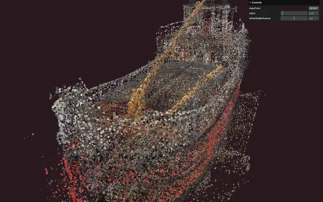
We’ve just created beautiful and perpetual chaos, but after a few seconds, we lose the shape of the boat.

We want the particles to live their life and, after a moment, get back to their initial position and start moving around again.

Each particle will have its own life span, meaning that we need this data to persist.

If only we had a value in addition to the rgb values… You guessed it, we are going to use the alpha channel.

Decay

For each particle, its life will start with an a to 0.0, it will increase with each frame and, when reaching 1, it will reset itself to the initial position and have its a back to 0.0, ready to start again.

In gpgpu/particles.glsl, after updating the particle.xyz, increment the a by 0.01:

void main()
{
    // ...
    
    // Decay
    particle.a += 0.01;

    gl_FragColor = particle;
}

Now we are going to use a condition to establish whether or not the particle is dead, which is when particle.a reaches 1.0 or above.

If it’s dead, for now, we’ll just reset the a to 0.0 ; otherwise, we apply the flow field and the decay:

void main()
{
    // ...
    
    // Dead
    if(particle.a >= 1.0)
    {
        particle.a = 0.0;
    }

    // Alive
    else
    {
        // Flow field
        vec3 flowField = vec3(
            simplexNoise4d(vec4(particle.xyz + 0.0, time)),
            simplexNoise4d(vec4(particle.xyz + 1.0, time)),
            simplexNoise4d(vec4(particle.xyz + 2.0, time))
        );
        flowField = normalize(flowField);
        particle.xyz += flowField * 0.01;
        
        // Decay
        particle.a += 0.01;
    }

    gl_FragColor = particle;
}

Make sure to keep the gl_FragColor update outside of the if and else statements.

No difference yet, because all we do is revert the a back to 0.0 when the particle dies.

Reset

We now want to reset the position, but we don’t have access to the initial position. Even though in the first frame uParticles contains the initial positions, it gets updated after each compute().

To fix that, we are going to send the baseParticlesTexture (the texture containing the initial positions) as a new uniform.

In script.js, after creating the uTime uniform, create a uBase uniform with the Uniform class and send it the baseParticlesTexture:

// Uniforms
// ...
gpgpu.particlesVariable.material.uniforms.uBase = new THREE.Uniform(baseParticlesTexture)

In particles.glsl, retrieve the uBase uniform as a sampler2D:

uniform sampler2D uBase;

After retrieving the particle from uParticles, do the same for uBase and save it as a vec4 base:

void main()
{
    // ...
    vec4 particle = texture(uParticles, uv);
    vec4 base = texture(uBase, uv);
    // ...
}

We could have put the base in the if, but having it before will come in handy later.

In the if (when the particle dies), set the xyz of particle to base.xyz:

void main()
{
    // ...
    vec4 base = texture(uBase, uv);
    
    // Dead
    if(particle.a >= 1.0)
    {
        particle.a = 0.0;
        particle.xyz = base.xyz;
    }
    // ...
}

Randomize

All the particles are dying at the same time because they all start at 0, get updated with the same amount on each frame, and die together.

To fix that, when populating baseParticlesTexture, change the 0 we assign to the alpha channel as Math.random():

for(let i = 0; i < baseGeometry.count; i++)
{
    // ...
    baseParticlesTexture.image.data[i4 + 3] = Math.random()
}

A turbulent and mesmerizing chaos.

Fix the frame rate

An issue that some of you with high-frequency monitors might have seen, is that the particles are dying faster.

It’s because we increment the life by 0.01 with each frame, regardless of the frame rate.

We need to use the delta time.

Just like we sent the uTime to the particlesVariable material uniforms, send a uDeltaTime to 0:

// Uniforms
// ...
gpgpu.particlesVariable.material.uniforms.uDeltaTime = new THREE.Uniform(0)

In the tick, update the uDeltaTime.value and assign to it the deltaTime that is already calculated:

const tick = () =>
{
    // ...

    // GPGPU Update
    gpgpu.particlesVariable.material.uniforms.uTime.value = elapsedTime
    gpgpu.particlesVariable.material.uniforms.uDeltaTime.value = deltaTime
    // ...
}

In particles.glsl, retrieve the uDeltaTime uniform as a float:

uniform float uDeltaTime;

When applying the decay to particle.a, use the uDeltaTime and multiply it by 0.3 so that it’s not too slow:

void main()
{
    // ...

    // Alive
    else
    {
        // ...

        // Decay
        particle.a += uDeltaTime * 0.3;
    }

    // ...
}

And since we are here, we also need to use the uDeltaTime when applying the flowField to the particle.xyz so that they move at the same speed regardless of the frame rate. Multiply it by 0.5 so that it’s fast enough:

void main()
{
    // ...

    // Alive
    else
    {
        // ...
        particle.xyz += flowField * uDeltaTime * 0.5;

        // Decay
        particle.a += uDeltaTime * 0.3;
    }

    // ...
}

Fix the long frames

One final bug we need to fix is when we get a long frame.

Long frames happen when the computer freezes for a moment or when we leave the tab and come back after a few seconds:

Note that browsers handle tick updates differently when the tab is not active.

All the particles are synchronized because, for one frame, the uDeltaTime was huge, and they all died together. That’s almost romantic, but we need to fix it.

There are multiple solutions for this issue.

The most common one is to make sure that deltaTime never gets too big directly in JavaScript. I personally like to limit it to 1/30 of a second because 30FPS is considered as the minimal frame rate for a decent experience.

But we are not going to use this technique. Instead, we are going to use a modulo 1 when resetting the a channel. This way, if the a goes beyond 1.0, it’ll simply loop back to 0 plus what was left and never exceed 1.0:

void main()
{
    // ...
    
    // Dead
    if(particle.a >= 1.0)
    {
        particle.a = mod(particle.a, 1.0);
        // ...
    }

    // ...
}

Control the chaos 02:04:45

Currently, we apply the flow field on all particles at all times. Although it looks nice, it’s not subtle, and we can’t see the model anymore.

We want to apply the flow field only on parts of the model, and we want it to vary organically.

We are going to use another Simplex Noise.

In the else, right before the flowField, call a simplexNoise4d(), send it the base.xyz as the first three values, time + 1.0 as the fourth (so that it’s different from the other simplexNoise4d()) and save it as strength:

void main()
{
    // ...

    // Alive
    else
    {
        // Strength
        float strength = simplexNoise4d(vec4(base.xyz, time + 1.0));

        // ...
    }

    // ...
}

The Simplex Noise goes from -1.0 to +1.0 and we want something from 0.0 to 1.0. It’s also the opportunity to smooth the value with a smoothstep:

void main()
{
    // ...

    // Alive
    else
    {
        // Strength
        float strength = simplexNoise4d(vec4(base.xyz, time + 1.0));
        strength = smoothstep(- 1.0, 1.0, strength);

        // ...
    }

    // ...
}

We can finally use the strength when applying the flowField:

void main()
{
    // ...

    // Alive
    else
    {
        // ...
        particle.xyz += flowField * uDeltaTime * strength * 0.5;

        // ...
    }

    // ...
}

It’s working, but it’s barely noticeable because even if some parts are moving just slightly, everything is moving.

But thanks to the smoothstep, we can now control how much of the particles are affected by the flow field.

As an example, change the first parameter of smoothstep to 0.0:

void main()
{
    // ...

    // Alive
    else
    {
        // ...
        strength = smoothstep(0.0, 1.0, strength);

        // ...
    }

    // ...
}

The higher the value, the less particles affected.

Reduce the frequency of the strength by multiplying base.xyz by 0.2 so that we get bigger chunks being affected:

void main()
{
    // ...

    // Alive
    else
    {
        // Strength
        float strength = simplexNoise4d(vec4(base.xyz * 0.2, time + 1.0));
        // ...
    }

    // ...
}

Tweak

Since we can control the number of particles affected by the flow field using the smoothstep, let’s add it to the debug panel.

We want a tweak from 0 to 1 where 0 results in no particle affected and 1 results in all particles affected.

In the particlesVariable uniforms, add a uFlowFieldInfluence uniform using Uniform and set it to 0.5:

// Uniforms
// ...
gpgpu.particlesVariable.material.uniforms.uFlowFieldInfluence = new THREE.Uniform(0.5)

In the Tweaks section, add one tweak for the 'value' of uFlowFieldInfluence from 0 to 1:

/**
 * Tweaks
 */
// ...
gui.add(gpgpu.particlesVariable.material.uniforms.uFlowFieldInfluence, 'value').min(0).max(1).step(0.001).name('uFlowfieldInfluence')

In particles.glsl, retrieve the uFlowFieldInfluence uniform as a float:

uniform float uFlowFieldInfluence;

The uFlowFieldInfluence is going from 0 to 1 and, when it does, we want the first parameter of the smoothstep to go from +1 to -1. It’s not the same range and it’s inverted.

We could use a remap function, but the formula isn’t that complicated.

Right before the smoothstep, create a float influence variable, subtract 0.5 from uFlowFieldInfluence so that it goes from -0.5 to +0.5, multiply it by -2.0 so that it goes from +1.0 to -1.0, use it in the first parameter of smoothstep:

void main()
{
    // ...

    // Alive
    else
    {
        // Strength
        // ...
        float influence = (uFlowFieldInfluence - 0.5) * (- 2.0);
        strength = smoothstep(influence, 1.0, strength);
        // ...
    }

    // ...
}

Life size 02:13:15

When dying, particles immediately pop back to their original position.

We want to control their size so that they grow up slowly, stay big for a moment, and start to shrink down before dying.

And to make the animation feel better, we want to make it smoother:

It’s very similar to what we did in the Fireworks lesson and we need to do it in particles/vertex.glsl (not gpgpu/particles.glsl).

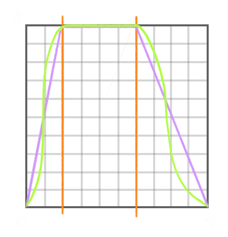
We can use the particle.a on a smoothstep to create a float sizeIn variable corresponding to when the particle scales up.

Then we use the particle.a on a smoothstep to create a float sizeOut variable corresponding to when the particle scales down.

Finally, we calculate the minimum of the two using min, save it as a size variable, and multiply it on gl_PointSize:

void main()
{
    // ...

    // Point size
    float sizeIn = smoothstep(0.0, 0.1, particle.a);
    float sizeOut = 1.0 - smoothstep(0.7, 1.0, particle.a);
    float size = min(sizeIn, sizeOut);

    gl_PointSize = size * aSize * uSize * uResolution.y;
    // ...
}

Final tweak 02:16:31

Our flow field animation is done, but let’s add a few improvements.

Hide the debug

First, let’s get rid of the debug plane.

Add a visible property to false in the gpgpu.debug Mesh:

gpgpu.debug.visible = false

Flow field strength tweak

We already have a tweak for the flow field influence.

Let’s add one for the flow field strength.

On the particlesVariable uniforms, add a uFlowFieldStrength uniform using the Uniform class and set it to 2:

// Uniforms
// ...
gpgpu.particlesVariable.material.uniforms.uFlowFieldStrength = new THREE.Uniform(2)

In the Tweaks section, add a tweak for it, with the min set to 0 and the max set to 10:

/**
 * Tweaks
 */
// ...
gui.add(gpgpu.particlesVariable.material.uniforms.uFlowFieldStrength, 'value').min(0).max(10).step(0.001).name('uFlowfieldStrength')

In gpgpu/particles.glsl, retrieve the uFlowFieldStrength uniform as a float and use it when adding the flowField to particle.xyz instead of 0.5:

// ...
uniform float uFlowFieldStrength;

// ...

void main()
{
    // ...

    // Alive
    else
    {
        // ...
        particle.xyz += flowField * uDeltaTime * strength * uFlowFieldStrength;
        
        // ...
    }

    // ...
}

Flow field frequency tweak

Just like we added a control for the strength, we can add a control for the flow field frequency.

To the particlesVariable uniforms, add a uFlowFieldFrequency uniform using Uniform and set it to 0.5:

// Uniforms
// ...
gpgpu.particlesVariable.material.uniforms.uFlowFieldFrequency = new THREE.Uniform(0.5)

In the Tweaks section, add a tweak for uFlowFieldFrequency with a min set to 0 and a max set to 1:

/**
 * Tweaks
 */
// ...
gui.add(gpgpu.particlesVariable.material.uniforms.uFlowFieldFrequency, 'value').min(0).max(1).step(0.001).name('uFlowfieldFrequency')

In gpgpu/particles.glsl, retrieve the uFlowFieldFrequency uniform as a float and multiply it in the particle.xyz when calculating the flowField:

// ...
uniform float uFlowFieldFrequency;

// ...

void main()
{
    // ...

    // Alive
    else
    {
        // ...
        vec3 flowField = vec3(
            simplexNoise4d(vec4(particle.xyz * uFlowFieldFrequency + 0.0, time)),
            simplexNoise4d(vec4(particle.xyz * uFlowFieldFrequency + 1.0, time)),
            simplexNoise4d(vec4(particle.xyz * uFlowFieldFrequency + 2.0, time))
        );
        
        // ...
    }

    // ...
}

Going further 02:20:29

And that’s it for the lesson.

As always, feel free to go further. Here are some suggestions:

• Add more tweaks. You can control the time frequency, the decay, the influence frequency, etc.
• Test with other models. Be careful, the model needs to be adapted to the effect with a lot of well-spread vertices.
• Give a global direction to the flowField, like in Chartogne Taillet where the particles seem to be pushed upward.
• Improve the look of the particles with something more fancy than the discs.
• Control the effect according to the cursor. Be careful, this one is a little bit tricky.